What panel Is Time Complexity?
Time complexity is the computational complexity useful in characterising the time required to execute an algorithm in terms of the size of the input. It gives an upper estimate of time that may be spent to perform a task and assists in evaluating how efficient various algorithms are.
Put very simply, time complexity is a measure of how an algorithm will run as the input size gets bigger.
As an example, consider an algorithm that has `O(n)` time complexity, then the time to run this algorithm on an input size that doubles in size will increase by approximately a factor of two. In the case of `O(n 2 )`, the time complexity, the execution time will increase four times when the size of the input doubles.
Why Does the Complexity of a Time Matter?
The importance of time complexity has to do with a number of reasons:
1. Performance Evaluation: It can aid us to determine the performance of an algorithm when it has become large.
2. Optimization: the analysis of time complexity is important since it allows developers to select or even create faster and more efficient algorithms.
3. Resource management: efficient algorithms give better performance in systems that have limited computational power or memory.
4. Preparation: Time complexity is a red-hot topic in coding competitions, and technical interviews.
It is the Big O Notation.
Big O notation defines the worst-case scenario (i.e. the longest the algorithm can run), and is by far the most common expression of time complexity.
A brief description of the most typical Big O notations can be seen as below:
Copy Code
Big O Notation | Name | Description |

---

O(1)           | Constant time     | The time does not grow with the size of input       |

O(log n)    | Log time  | The time performs in a logarithmic manner to the input   |

O(n)             | O(n) time           | Time is proportional to the input           |

O(n log n)  | Linearithmic | A little bit worse than linear, quite common in sports  |

O(n 2 )        | Quadratic time  | The time algorithm grows with the n 2 of the input |

O (2 )  | Exponential-time algorithm  | Time increases every time a new input is given by a factor of doubling     |

O ( n!)Time in factorial O(n!), Extremely slow and is used in permutations |
Now we are going to take a closer look at each of them trying to exemplify it.
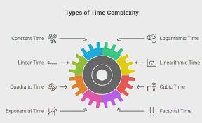
General Time Complexities and example
1. Constant Time – O(1)
Constant time An algorithm is said to have constant time complexity when it does not need to depend on the size of the input data to execute.
Example:
Copy Code
```cpp

int getFirstElement(int arr[])

    return arr[0];

}

```
This function always takes the same length of time regardless of the size of the array.
Real world analogy: Grabbing a book off a shelf without caring the number of books in the shelf.
2. Logarithmic Time – O(log n)
Algorithm Algorithms that reduce the size of the problem by a factor of two at each step run in logarithmic time.
E.g. Binary Search
Copy Code
cpp

int binarySearch(int arr[ ], int x, int low, int high) {

    w h i l e (l o w l e q g e q q g e t t s n k o i d s ) {

        int mid = ( low + high ) / 2;

        if (arr[mid]= x)

            return mid;

        or else ( x )when are[mid] < x

            low = mid+1;

        else

            high = mid -1;

    }

    return -1;

}
Every time, binary search cuts the search space into two. It will therefore run in O(log n).
Real life analogy: Finding a word in a dictionary by turning to half the pages of a dictionary.
3. Linear Time – O(n)
In a linear time algorithm, the time increases linearly with the input size.
Example:
Copy Code
cpp

int sum(int arr[ ], int n) {

    int total = 0;

    for (int i = 0; i< n; i++)

        total = total + arr[i];

    return total;

}
In this case, every object is revisited.
Real life analogy example: Taking a role call of all names in a list.
4. Linearithmic Time - O (n log n)
This is a combination of both the linear and logarithmic complexities. Such algorithms include those that do linear work per logarithmic division.
Example: Merge Sort.
Copy Code
cpp

void mergeSort(int arr[], int l, int r)

    if (l = =r)

        return;

    int mid = l + (r-l)/ 2;

    mergeSort(arr;l;mid);

    mergeSort(arr, mid +1, r);

    tomerge(arr, l, mid, r);

}
The algorithm of merge sort breaks the array log n (n times) and merges the divisions (log n times) leading to O (n log n).
Real-life analogy: playing with a deck of cards: Taking a deck of cards that is mixed up and by using divide and conquer, sorting the deck out.
5. Оквадратичное – O(n²)
Time scales as a square of the size of the input. Such are not very effective when inputs are big.
Example: Selection Sort
Copy Code
cpp

void bubbleSort(int arr[], int n)

    for (int i = 0; i < n - 2; i++)

        for (int j = 0; j  - i - 1; j++)

            when (arr[j] > arr[j + 1])

                swap(arr[j + 1, arr[j]]);

}
The two loops are nested, the two loops are conditional on n and hence the value of n squared is nn = n 2.
Real life analogy: To compare the pairs of the students in a single table and identify the tallest student amongst the two.
6. Cubic Time- O (n 3)
It occurs when there are three levels of loop nesting and time required is proportional to the cube of the input size.
Example:
Copy Code
cpp

void tripleLoop(int n)

    for (int i = 0; i < n;{i

        for (int j = 0; j < n; j++)

            type type.Comparing(String s1, String s2) { return 0; } }

                cout << i << j << k << " \n";

}
Even slower on the scale of time complexity is cubic, which is usually avoided.
7. Exponential Time O (2 ^ n )
This is a time complexity which is observed in algorithms whose complexity is by exploring all subs and combinations.
Example: Recursive Fibonacci Series
Copy Code
cpp

int fibonacci(int num) {

    if (n= 1)

        return n;

    return fibonacci( n - 1 ) + fibonacci ( n - 2 );

}
Every call is calling two additional calls, which begins exponentially.
Real example analogy: Feeling every possible combination of keys in order to open a lock.
8. Order of Factorial Time = O (n!)
This is the poorest category and usually accompanied by brute-force type algorithms of permute basing systems.
On example: Traveling Salesman Problem (Brute Force)
The number of permutations in checking each of the possible pathways between cities is n!.
Real world analogy: Computing each and every possible configuration of the seating position of 10 people.
Best Case, Worst Case and Average Case
Time complexity Time complexity can be considered in worst case (Big O) and other notations are also helpful:
Best-case (O): Less work to be done.
Average-case (Theta): Implied time on average in all the inputs.
Say in the case of linear search:
This is in the best case O(1) when it is the first element.
Worst-case: O(n) in case the element is the last one or it is not there.
Time Complexity Calculation
This is a checklist in a nutshell:
1. Count the operations which are dependent on input size.
2. Disregard constants and terms of lower order (we concentrate attention on the principal term).
3. Here is one to find nested loops--root them out because each level compounds on the other.
4. Recursive algorithms can be used using recurrence relations.
Example:
Copy Code
cpp

void example(int n){

    for (int i = 0;i <n;i++) // O(n)

        for (int j = 0; j < n; j++) // n work

            cout << i << j // O(1)

}

Total time complexity O(n n ) = O(n 2)
Ways of Optimizing Time Complexity
1. Apply the effective data structures (such as HashMaps, Heaps).
2. Use nested loops when you need them but you should avoid it.
3. Use divisions and conquers.
4. Memoization and dynamic programming may be used to check on overlapping subproblems.
5. In cases where this is possible, make use of greedy algorithms.
Time Complexity Table: Cheatsheet
Complexity White box Input Size n = 10 n = 100 | n = 1000
Of course there is an identity of place, in such a way that there is an identity of place which will exist when I have lost myself.
Copy Code
| O(1)       | 1cmd             | 1           | 1           |

| O(log n)  | 3   | 7| 10          |

| O(n)  | 10                  | 100           | 1000        |

| O(n log n) | 33                 | 700           | 10.000      |

O(n 2 )      | 100                 | 10,000            | 1,000,000

O(2n)     | 1024

O (n!)     | 3.6 million   | Too big | Unimaginable
Conclusion
One of the foundations of algorithmic thinking is time complexity. It enables you to judge the goodness of scale of algorithms, pick the most cost efficient solution and extrapolate performance of large inputs. Time complexity is always a competitive advantage either during technical interviews or when you are optimizing code to run in production.
It is not merely a theoretical exercise, it is a practical one to learn the clever subtlety between O(1), O(n log n), or O(2 n ). The difference between the app that loads within a second or the one which crashes in real life is noticeable.