Shortest Paths Dijkstra Algorithm
The algorithm that is the backbone of history in graph algorithm is the Dijkstra algorithm, used to compute the shortest paths between nodes in a graph . In 1956 Edsger W. Dijkstra conceived it to address the issue of shortest paths between nodes. This algorithm operates on selecting any of the nodes and finding the minimum path, based on the source node to the rest of the nodes in the graph. It is especially helpful in, say, the GPS systems to decide on the least distance between any two places.
Comprehending the Fundamentals of Dijkstra Algorithm
Dijkstra algorithm is a sequence of steps involved in solving problems in a graph. Often the standard version of the algorithm pins one node as the source and finds the shortest paths outward this source to every other node in the graph. The algorithm acts on graphs, in which cities might be described as of vertices, and the route might be described as the edges. It is a greedy algorithm, that is, it makes locally optimal decisions at every step and then hopesto reach a global optimum, and it fails to work properly when edges have negative weights.
The way Dijkstra Algorithm Works
The steps of Dijkstra algorithm can briefly be reduced to the following steps:
Initialization: The algorithm is set off with a given node (the source) and finds the shortest path between that node and any other node on the graph. It initializes an array, usually called dist, with an infinite value except on the source node which is initialized to 0. Moreover, there is an initialization of a prev array to UNDEFINED of all the vertices.
Distance Calculation: The algorithm computes successively the shortest distance of each node with the source. When a shorter path is discovered than a path recorded, the new shortest distance replaces it.
Node Marking: Shortest path to any other node is computed, and then that particular node is marked as visited. This eliminates the possibility of an infinite loop that the algorithm creates by reprocessing the already visited nodes.
Iteration: Distance calculation and marking of the nodes are repeated until one is able to visit all the nodes in the graph. This is done such that the nearest route to all the accessible nodes that are reachable origin is identified and stored.
These steps can be illustrated by these lines on the pseudocode of the algorithm:
Copy Code
function Dijkstra(Graph, source) ((16))

  for each vertex v in Graph.Vertices: ((17))

    dist ← INFINITY ((18))

    prev ← UNDEFINED ((19))

  dist ← 0 ((20))

  while Q is not empty: ((21))

    u ← vertex in Q with min dist ((22))

    for each neighbor v of u still in Q: ((23))

      alt ← dist + Graph.Edges(u, v) ((24))

      if alt < dist: ((25))

        dist ← alt

        prev ← u

  return dist, prev ((26))
The algorithm can be applied differently, e.g. by returning an array, employing a priority queue or by optimizing to infinite graphs.
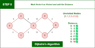
Pragmatical Demonstrations and Illustrations
In order to familiarize with the algorithm by Dijkstra better, one should resort to practice. As an example, the typical step by step demonstration is finding the shortest path between two nodes such as A and G. To know at which point a path changes, when the weights on the edges are changed can be explained visually intuitive by using visual means, when in each step the Dijkstra algorithm to find out shortest paths. These visualization may appear as animation or frozen graph for visual triangulation. As an example, graph representations apply to a real world map where Figure 3(a) can be used to represent the visual representation.
Computational Complexity
The time complexity of the algorithm of Dijkstra usually relates to how the algorithm is implemented. According to the given pseudo code, its time complexity is O(𝑛2n2 and the number of vertices is \(n\), denoted by \(n\). The space complexity is linear and O(\(n\)). On other analyses, Dijkstra algorithm has a time complexity of O(𝑉2 That is, in 0.22 seconds, (comparison)using O(The V+E) memory, it used 179,241 to 190,961 bytes. In large scale situations, Dijkstra algorithm, compared to other algorithms such as A-Star, may consume more memory and take repeated iterations.
How to Learn Dijkstra Algorithm with Uncodemy
Students that want to gain more experience and knowledge on Dijkstra algorithm and other similar ideas will have a chance to acquire them in a series of IT education courses provided by Uncodemy. Although particular courses strictly focused on learning Dijkstra algorithm are not mentioned, Uncodemy can be regarded as one of the most popular IT training institutes where it is possible to learn such topics as Data Science, Full Stack Development, Python, Java, Software Testing, Data Analytics, and Digital Marketing. Wider areas that tend to cover graph theory and implementation of algorithms are pertinent to the acquisition of Dijkstra algorithm in practice. Python is one of the examples of how learning the language will be of any use when using such algorithm as Dijkstra: there are step-by-step tutorials on doing it with Python.
Conclusion
The problem of shortest path in graphs is solved in an efficient way by the algorithm described by Dijkstra, which can be used in things like navigation systems as well as in network routing. It is a standard in the field of computer science and real-life situations because of its efficiency on finding optimum routes. Albut, although it is optimal, it is important to learn about the computational complexity of the same and deliberate limitations like its incapability to handle negative weights to enable their proper use. Individuals who would want to learn how to use such algorithms on a higher level should learn data structures and various programming languages thorougly.