This article will provide a comprehensive, student-friendly introduction to the most important distributions used in statistics, including the normal, binomial, Poisson, and several others. We will walk through their definitions, applications, differences, and relevance in data science so that by the end, you will have a solid foundation to apply them in practical situations.
Understanding Distributions in Statistics
A distribution in statistics refers to the way values in a dataset are spread across the possible range of outcomes. Imagine rolling a die: each number (1 through 6) has an equal chance of appearing. This predictable spread of outcomes is called a probability distribution because it assigns probabilities to all potential results. In contrast, real-world data often follows more complex patterns, which is why different statistical distributions are used to model different types of data.
The concept of distribution is essential because it underpins much of statistical analysis. By understanding the shape, center, and spread of data, you can determine what methods, models, or visualizations are appropriate. For students in a Data Science Course in Noida, mastering distributions provides the groundwork for tasks such as statistical testing, predictive modeling, anomaly detection, and more.
The Importance of Knowing Different Types of Distribution
Not all datasets follow the same pattern. Some datasets are symmetric, while others are skewed. Some show discrete jumps between possible values, while others flow smoothly. Some have fixed limits, and some can, at least theoretically, stretch infinitely. Using the wrong distributional assumption can lead to flawed analyses, biased predictions, and misleading conclusions.
Understanding the types of distribution helps you select the right statistical tools. For example, you would use the binomial distribution to model the number of times a coin lands heads in 10 tosses, but you would use the Poisson distribution to model the number of emails arriving in an hour. Similarly, the normal distribution is widely used in hypothesis testing and confidence intervals due to its well-defined properties.
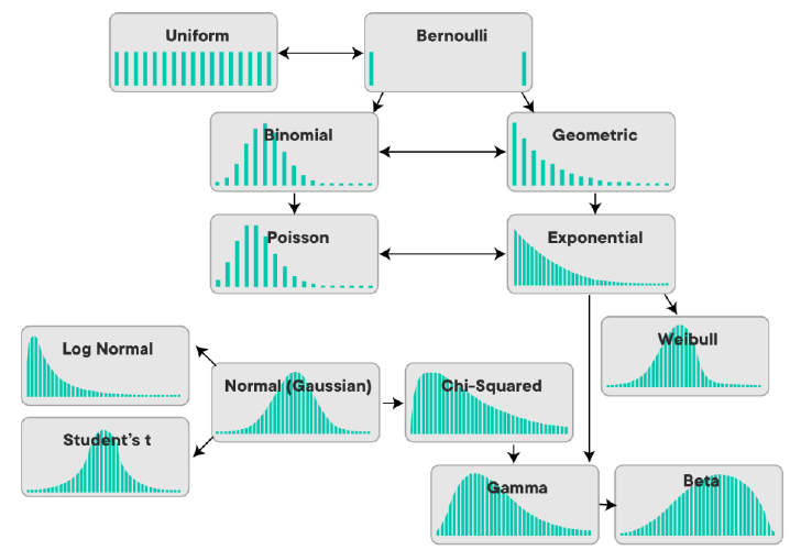
The key distributions that every beginner should understand are:
The Normal Distribution
The normal distribution, often referred to as the Gaussian distribution or bell curve, is the most well-known and widely used distribution in statistics. It describes a continuous, symmetric distribution where most observations cluster around the mean (average), and the likelihood of extreme values decreases as you move further away.
Mathematically, the normal distribution is defined by two parameters: the mean (μ), which determines the center, and the standard deviation (σ), which controls the spread. In a perfectly normal distribution, about 68% of the data falls within one standard deviation of the mean, about 95% within two, and about 99.7% within three — a rule known as the empirical rule.
Applications of the normal distribution are everywhere: heights, weights, IQ scores, blood pressure readings, standardized test scores, and even measurement errors often follow this pattern. In data science, the normal distribution underpins many statistical tests (such as the t-test and z-test) and serves as the backbone of numerous models and machine learning algorithms.
Students enrolled in a Data Science Course in Noida will work extensively with the normal distribution, learning how to standardize data (using z-scores), check for normality in datasets, and apply tests that assume normality. Understanding when and why data is normally distributed is fundamental for any data scientist.
The Binomial Distribution
While the normal distribution models continuous outcomes, the binomial distribution deals with discrete events — specifically, the number of successes in a fixed number of independent trials, each with the same probability of success. Imagine flipping a coin 10 times: the binomial distribution models the probability of getting, say, exactly 6 heads.
The binomial distribution is defined by two parameters: the number of trials (n) and the probability of success (p) in each trial. For example, if you are testing a new drug and each patient has a 70% chance of recovery, the binomial distribution can model how many out of 20 patients you can expect to recover.
Key characteristics of the binomial distribution include its discreteness (it only takes whole-number values) and its symmetry or skewness, which depends on the value of p. When p = 0.5, the distribution is symmetric, but when p moves closer to 0 or 1, the distribution becomes skewed.
For students taking a Data Science Course in Noida, understanding the binomial distribution is crucial when working with categorical or binary data. Common use cases include modeling success/failure outcomes, estimating conversion rates, analyzing customer churn, or evaluating A/B test results.
The Poisson Distribution
The Poisson distribution is another discrete distribution, but unlike the binomial distribution, it models the number of events occurring in a fixed interval of time or space, where events happen independently and at a constant average rate. For example, you might use the Poisson distribution to model the number of calls arriving at a call center in an hour or the number of typos in a book.
The Poisson distribution is characterized by a single parameter, λ (lambda), which represents the average rate of occurrence. One of its most interesting features is that the mean and variance are equal (both equal to λ), which makes it easy to check if data fits a Poisson pattern.
Common applications include modeling traffic accidents, network packet arrivals, customer service queues, or rare disease occurrences. In data science, Poisson models are often used in operations research, web analytics, and text mining.
Students in a Data Science Course in Noida will likely encounter Poisson regression, an extension of the Poisson distribution used to model count data with predictors, providing a powerful tool for predictive analytics.
The Exponential Distribution
Closely related to the Poisson distribution is the exponential distribution, which models the time between successive events in a Poisson process. For example, if the number of buses arriving at a stop per hour follows a Poisson distribution, then the time between two buses follows an exponential distribution.
The exponential distribution is defined by its rate parameter, often denoted by λ. It has a memoryless property, meaning the probability of an event occurring in the next interval does not depend on how much time has already passed.
Applications include modeling waiting times, survival analysis, and reliability engineering. In data science, the exponential distribution helps estimate system uptime, machine failure rates, and customer inter-arrival times.
Understanding the relationship between the Poisson and exponential distributions gives students in a Data Science Course in Noida a deeper grasp of stochastic processes and queueing theory.
The Uniform Distribution
The uniform distribution is one of the simplest continuous distributions. It models a situation where all outcomes in a given range are equally likely. For example, if you generate a random number between 0 and 1, the uniform distribution ensures that every number in this interval has the same probability.
There are two types of uniform distributions: discrete uniform (where a finite number of outcomes are equally likely) and continuous uniform (where any value within a range is equally likely).
Applications include random sampling, Monte Carlo simulations, and initializing weights in machine learning models. While simple, the uniform distribution plays a foundational role in probabilistic modeling and random number generation, topics that students in a Data Science Course in Noida will encounter frequently.
The Bernoulli Distribution
The Bernoulli distribution is the simplest discrete distribution, modeling a single trial with two possible outcomes: success (1) or failure (0), with probability p of success. It can be thought of as the building block of the binomial distribution, which models multiple Bernoulli trials.
Applications include modeling binary outcomes such as yes/no decisions, click/no-click events, or defective/non-defective products. In machine learning, the Bernoulli distribution appears in logistic regression, Naive Bayes classifiers, and probabilistic models for binary data.
Students in a Data Science Course in Noida should understand how Bernoulli trials combine into more complex distributions and models, reinforcing the connection between simple probability and sophisticated analysis.
Comparing the Distributions
While each distribution has its specific use cases, it is important to understand how they relate and differ. For example, the binomial and Poisson distributions both model counts, but the binomial has a fixed number of trials, while the Poisson has no fixed upper limit. The normal distribution models continuous outcomes and serves as a limiting case for many discrete distributions when the number of trials is large (a result known as the Central Limit Theorem).
Knowing which distribution to apply depends on the data’s nature (discrete or continuous), the underlying process (fixed trials or constant rate), and the questions being asked (probabilities, averages, waiting times, etc.). Students in a Data Science Course in Noida will practice identifying these situations and applying the right tools accordingly.
Conclusion
Mastering the types of distribution is essential for any aspiring data scientist, analyst, or researcher. Whether you are modeling customer behavior, forecasting sales, detecting anomalies, or designing experiments, knowing how data is distributed provides the foundation for sound statistical reasoning and effective decision-making.
In this article, we explored the most important distributions used in statistics: the normal, binomial, Poisson, exponential, uniform, and Bernoulli distributions. We covered their definitions, key properties, and real-world applications, all within the context of data science. For students enrolled in a Data Science Course in Noida, this knowledge will be invaluable as you progress through advanced topics like hypothesis testing, regression modeling, machine learning, and time series forecasting.
Remember, statistical distributions are not just abstract mathematical concepts; they are practical tools that allow us to make sense of uncertainty, variability, and randomness in the real world. By understanding their assumptions, strengths, and limitations, you can become a more effective and insightful data practitioner.